The Math of SRE Explained: SLI and SLOs
Statistics 101 and Extreme Value Theory
Let me share what I've learned from 12 years of experience, defining and defending SLOs on various software and hardware systems, including TPU pods, HPC/GPU clusters, and general compute clusters. (This is just an introductory post, but I need to cover the basics before diving into more juicy topics)
SRE, by the book, defines SLI as "quantitative measure of some aspects of the level of a service that is provided" and SLO as " a target value or range of values for a service level that is measured by an SLI"; the SRE workbook warns that "It can be tempting to try to math your way out of these problems [...] Unless each of these dependencies and failure patterns is carefully enumerated and accounted for, any such calculations will be deceptive".
I agree with the last statement, but let's not shy away from the journey. Let's embrace math, and we'll uncover a rich and fascinating landscape.
Fantastic SLIs/SLOs and where to find them
Here is a bestiary of SLIs and SLOs commonly found in the wild, to lay the ground of what we'll be talking about.
SLIs for software services usually cover latency, which is the time it takes to respond to a request or finish a task, error rate, the ratio of failed requests to total requests received, and some measure of system throughput, like requests per second or GBps.
Not all requests are created equal. It's common to set different SLOs for different types or classes of requests. Various terms – such as priority, criticality, or quality of service (QoS) – are used in different situations, but they all serve the purpose of treating requests differently and managing load when a service is under stress.
Compute services, such as Kubernetes clusters or Borg cells, operate on a different time scale compared to web services, but they are not entirely different. Users care about how long it takes to schedule a job (or to receive an error), that scheduling failures are rare, and how efficiently compute resources are used compared to the theoretical zero-overhead scenario.
For both software services and compute resources, it's common to define availability.
In systems that show measurable progress, we focus on the portion of throughput that is truly effective. This concept of application-level throughput is known as goodput in networking, and the term has also been embraced by ML (at least at Google).
In storage systems, we also care about durability, which is the likelihood of accurately reading back what we wrote without any errors or silent corruption.
Given enough size, silent data corruption is also a problem that you care about in compute infrastructure.
SLIs are usually defined as a certain quantile over a sample or measurement, and these quantiles often fall at the tail of distributions, not in the center. This is an important point because it changes the mathematical rules of the game!
Perfection is costly. It is common to define SLI as the latency of 95/99% of requests, and you rarely or never see max latency in SLO definitions. When it does appear, there are always escape clauses.
Most hyperscaler services and the business scenarios they support aim for between 3 (99.9%) to 5 (99.999%) nines of availability. However, many users can tolerate even less at the instance- or region-level, e.g. with 99% availability allowing for up to 7.2 hours of downtime per month.
There are users in the world who can't tolerate more than 30 milliseconds of server downtime per year. They require 99.9999999% availability, and there are systems capable of delivering these impressive numbers. However, this level of reliability is not typical for common computing infrastructure. (For those interested, the number above is the stated reliability of an IBM z16 mainframe.)
A side trip into probability distribution and basic statistics
If you're already familiar with basic frequentist versus Bayesian statistics, distribution families, and the central limit theorem, feel free to skip this section.
If you're not familiar or just want a refresher, let's start with the basics. We'll discuss counting things, as we aim to measure how often a system fails.
A random variable is a variable with a value that is uncertain and determined by random events. In mathematical terms, it's not actually a variable, but a function that maps possible outcomes in a sample space to a measurable space (known as the support).
So, when the possible outcomes are discrete and finite or countably infinitely many outcomes or uncountably infinite (and piecewise continuous), we can define the expectation of a random variable X respectively as:
$$\begin{align*} E[X] &= x_1p_1+x_2p_2+\dots+x_kp_k\\ E[X] &= \sum_{i=1}^{\infty}x_ip_i \\ E[X] &= \int_{-\infty}^{\infty}xf(x)dx \end{align*}$$
where p_i is the probability of outcome x_i and f(x) is the probability density function (the corresponding name in the discrete case – i.e. pmf(x_i)=p_i – is called the probability mass function).
There are two main approaches to statistics.
Frequentist or classical statistics, assigns probability to data, focusing on the frequency of events, and tests yield results that are either true or false.
Bayesian statistics, assigns probabilities to hypotheses, producing credible intervals and the probability that a hypothesis is true or false; it also incorporates prior knowledge into the analysis, updating this as more data becomes available.
Probability distributions aren't isolated; they are connected to each other in complex ways. They can be transformations, combinations, approximations (for example, from discrete to continuous), or compositions of each other, and so on...
The binary outcome {0, 1}, like available/broken, of independent events is a Bernoulli random variable (rv) with parameter p, which represents the probability of events. When we sample from a Bernoulli distribution, we get a set of values that can either be 0 or 1.
When counting events in discrete time, such as if we consider events that fall in a given second/minute/hour/month:
The time between positive events follows a Geometric distribution with the same parameter p;
The time between every second positive event follows a Negative Binomial distribution with the same success probability p as before and r=2, meaning we are focusing on every second positive event.
- An notable point is that the Negative Binomial random variable is the sum of Geometric random variables.
The number of events in a given interval or sample of size N follows a Binomial distribution with parameters p and N.
- For instance, the raw number of available TPU slices in a TPUv2 or v3 pod, or the number of DGX systems in a DGX Superpod, can be roughly estimated using this distribution... but what makes the difference in these systems is how you manage disruptions, planned and unplanned maintenance.
When we start counting events in continuous time, we discover matching distributions with the same mathematical structure and relationships. These are the limit distributions of the previous ones when the interval sizes become infinitely small. For those who are particularly adventurous, let me mention that category theory offers an alternative and much broader explanation, as is often the case.
The time between independent events happening at a constant average rate and with a probability p follows an Exponential random variable with a rate parameter λ=1/p.
The time between every k-th event follows a Gamma random variable with parameters k and θ=1/p.
- The Gamma random variable is the sum of k exponential random variables, the same relationship as the negative binomial and geometric random variables above.
The number of events in a given time span of size N is a Poisson random variable with rate parameter λ=N/p.
We refer to a "sample" as a subset of values taken from a statistical population. A "sample statistic" is a value calculated from the sample. When we use a statistic to estimate a population parameter, we call it an "estimator".
For a sufficiently large number of events in Bernoulli samples, if we count the number of positive events and divide by the total number of events, the result will be close to p. As the number of events grows to infinity, the result converges to p, which is the "mean" of the Bernoulli distribution. This is known as the "law of large numbers": the average obtained from a large number of i.i.d. random samples converges to the true value if it exists.
The average of many samples of a random variable, which has a finite mean and variance, becomes a random variable that follows a Normal distribution, under specific conditions. This is known as the "central limit theorem".
This is what most people recall from their introductory statistics courses.
The central limit theorem, need not apply... Extreme Value Theory
Let's talk about when the central limit theorem does not apply, as this is a common situation with the data that SREs deal with. Not knowing its limits is one reason why relying on what people remember from introductory statistics is discouraged (though it's not the only reason).
A popular way to normalize data is to compute the Z-score, defined as:
$$Z = {{x - \mu} \over {\sigma}}$$
where Z is known as the standard score, and it normalizes samples in terms of standard deviations (σ) and the mean (μ).
But don't attempt to analyze variability in error rates by normalizing error and request counts, and then calculating the ratio. The ratio of two independent Normal random variables with a mean of zero (Cauchy random variables) has an undefined mean!
There are two other crucial distributions that frequently appear in SLI and SLO, yet many SREs seem unaware of them. These distributions are connected to quantiles and significant deviations from the median of a probability distribution. Therefore, the field of statistics that examines them is known as Extreme Value Theory.
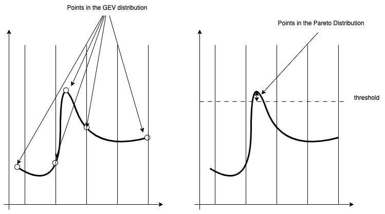
There are two primary methods for analyzing the tails of distributions.
You can calculate the maximum or minimum values over a specific period or block, and then analyze the distribution of these values (for example, the highest values of each year based on the highest values of each month). This method helps you understand the distribution of the minimum or maximum values from very large sets of identical, independently distributed random variables from the same distribution. The distribution you find is often a form of the Generalized Extreme Value Distribution. Here we consider the maxima/minima and then compute the distribution that it follows given a arbitrarily large or infinity amount of time. It's good to estimate the worst-case scenario for a steady-state process.
You can count how many times peak values go above or below a certain threshold within any period. There are two distributions to look at: the number of events in a specific period (like a Poisson distribution mentioned earlier), and how much the values exceed the threshold, which usually follows a generalized Pareto distribution. Here we consider the frequency of violations and how severe they can be.